Python Tutorial
For more detailes about artm.LDA, artm.ARTM, artm.BatchVectorizer and artm.Dictionary see Python Interface and Python Guide.
LDA (most simple)
artm.LDA was designed for non-advanced users with minimal knowledge about topic modeling and ARTM. It is a cutted version of artm.ARTM model with pre-defined scores and regularizers. artm.LDA has enough abilities for fitting the LDA with regularizers of smoothing/sparsing of  and
and  matrices with offline or online algorithms. Also it can compute scores of perplexity, matrices sparsities and most probable tokens in each topic, and return the whole resulting matrices.
Let’s make a simple model experiment with ‘kos’ collection in UCI format (see Input Data Formats and Datasets). You will need two files: docword.kos.txt и vocab.kos.txt. Both these files should be put into the same directory with this notebook. Let’s import the artm module, create BatchVectorizer and run dictionary gathering inside of it (if you are interested in the detailes, you need to read information from given links):
import artm

batch_vectorizer = artm.BatchVectorizer(data_path='.', data_format='bow_uci',
                                        collection_name='kos', target_folder='kos_batches')
Now let’s create the model by defining the number of topics, number of passes through each document, hyperparameters of smoothing of and and dictionary to use. Also let’s ask thr model to store matrix to have an ability to look at it in the future.
Also you can set here the num_processors parameter, which defines the number of threads to be used on your machine for parallelizing the computing:
lda = artm.LDA(num_topics=15, alpha=0.01, beta=0.001, cache_theta=True,
               num_document_passes=5, dictionary=batch_vectorizer.dictionary)
Well, let’s run the learning process using offline algorithm:
lda.fit_offline(batch_vectorizer=batch_vectorizer, num_collection_passes=10)
That’s all, the fitting is over. You can iterate this process, edit model parameters etc. Now you are able to look at the results of modeling. For instance, let’s look at final values of matrices sparsities:
lda.sparsity_phi_last_value
lda.sparsity_theta_last_value
Or at all values of perplexity (e.g. on each collection pass):
lda.perplexity_value
You can see the most probable tokens in each topic, at last. The are returned as list of lists of strings (each internal list correspondes to on topic by order). Let’s output them with pre-formatting:
top_tokens = lda.get_top_tokens(num_tokens=10)
for i, token_list in enumerate(top_tokens):
     print 'Topic #{0}: {1}'.format(i, token_list)
To get the matrices you can use th following calls:
phi = lda.phi_
theta = lda.get_theta()
Here’s two more abilities of artm.LDA.
At first, it is the ability to create matrix for new documents after the model was fitted:
batch_vectorizer = artm.BatchVectorizer(data_path='kos_batches_test')
theta_test = lda.transform(batch_vectorizer=test_batch_vectorizer)
Secondly, in the case, when you need a custom regularization of each topic in matrix, you need to set beta a list instead of scalar value. The list should have th length equal to the number of topics, and then each topic will be regularized with corresponding coefficient:
beta = [0.1] * num_topics  # change as you need
lda = artm.LDA(num_topics=15, alpha=0.01, beta=beta, num_document_passes=5,
               dictionary=batch_vectorizer.dictionary, cache_theta=True)
ARTM
This is a simple example of usage of artm.ARTM, a full-power Python API for BigARTM library. Let’s learn two topic models of text collections, ARTM and PLSA, and compare them.
One of the important measures is the perplexity. Nevertheless it’s not the only way to chech the quality of the model learning. The list of implemented scores can be found in Scores Description and there interfaces are described in Scores. We’ll use perplexity, sparsities of and , topic kernel scores (the higher values of sparsities and average purity and contrast means the more interpretable model).
The goal of the experiment is to learn the ARTM model in the way to obtain better values of sparsities and kernel characteristics, than in PLSA, without significant decline of the perplexity.
The main tool to control the learning process is the regularization. The list of currently implemented regularizers can be found in Regularizers Description and there interfaces are described in Regularizers. We will use SmoothSparsePhi, SmoothSparseTheta and DecorrelationPhi regularizers. ARTM without the regularization corresponds the PLSA model.
Let’s use the same ‘kos’ collection, that was described above. At first let’s import all necessary modules (make sure you have the BigARTM Python API in your PATH variable):
%matplotlib inline
import glob
import os
import matplotlib.pyplot as plt

import artm
Library Python API similarly to scikit-learn algorithms represents input data in the form of one class called BatchVectorizer. This class object get batches or UCI / VW files or  matrix as inputs and is used as input parameter in all methods. If the given data is not batches, the object will create them and store to disk.
So let’s create the object of artm.BatchVectorizer:
batch_vectorizer = None
if len(glob.glob(os.path.join('kos', '*.batch'))) < 1:
    batch_vectorizer = artm.BatchVectorizer(data_path='', data_format='bow_uci',
                                            collection_name='kos', target_folder='kos')
else:
    batch_vectorizer = artm.BatchVectorizer(data_path='kos', data_format='batches')
ARTM is a class, that represents BigARTM Python API. Allows to use almost all library abilities in scikit-learn style. Let’s create two topic models for our experiments. The most important parameter of the model is the number of topics. Optionally the user can define the list of regularizers and quality measures (scores) to be used in this model. This step can be done later. Note, that each model defines its own namespace for names of regularizers and scores.
dictionary = batch_vectorizer.dictionary
topic_names = ['topic_{}'.format(i) for i in xrange(15)]

model_plsa = artm.ARTM(topic_names=topic_names, cache_theta=True,
                       scores=[artm.PerplexityScore(name='PerplexityScore',
                                                    dictionary=dictionary)])

model_artm = artm.ARTM(topic_names=topic_names, cache_theta=True,
                       scores=[artm.PerplexityScore(name='PerplexityScore',
                                                    dictionary=dictionary)],
                       regularizers=[artm.SmoothSparseThetaRegularizer(name='SparseTheta',
                                                                       tau=-0.15)])
Dictionary is the object of BigARTM, containing the information about the collection (vocabulary, different counters and values, linked to tokens). Provided dictionary will be used for matrix initialization. It means:
- the matrix with the name ‘pwt’ will be created with numbers of rows and columns corresponding the numbers of tokens in the dictionary and topics in the model;
- this matrix will be filled with random values from (0, 1) and normalized.
Matrix will be initialized during first call of ARTM.fit_offline() or ARTM.fit_online().
As it was said earlier, ARTM provides the ability to use all the scores of BigARTM. Once the score was included into model, the model will save all its values, obtained at the time of each matrix update. Let’s add the scores we need for our experiment (only ones, missed in the constructors):
model_plsa.scores.add(artm.SparsityPhiScore(name='SparsityPhiScore'))
model_plsa.scores.add(artm.SparsityThetaScore(name='SparsityThetaScore'))
model_plsa.scores.add(artm.TopicKernelScore(name='TopicKernelScore',
                                            probability_mass_threshold=0.3))

model_artm.scores.add(artm.SparsityPhiScore(name='SparsityPhiScore'))
model_artm.scores.add(artm.SparsityThetaScore(name='SparsityThetaScore'))
model_artm.scores.add(artm.TopicKernelScore(name='TopicKernelScore',
                                                  probability_mass_threshold=0.3))
Now we’ll do the same thing with the regularizers for artm_model (let’s set their start coefficients of the regularization, these values can be changed later):
model_artm.regularizers.add(artm.SmoothSparsePhiRegularizer(name='SparsePhi', tau=-0.1))
model_artm.regularizers.add(artm.DecorrelatorPhiRegularizer(name='DecorrelatorPhi', tau=1.5e+5))
Now we’ll try to learn the model in offline mode (e.g. with one matrix update during one path through the whole collection). Let’s start with 15 passes:
model_plsa.num_document_passes = 1
model_artm.num_document_passes = 1

model_plsa.fit_offline(batch_vectorizer=batch_vectorizer, num_collection_passes=15)
model_artm.fit_offline(batch_vectorizer=batch_vectorizer, num_collection_passes=15)
Let’s check the results of first part of learning process by comparing the values of scores of both models:
def print_measures(model_plsa, model_artm):
    print 'Sparsity Phi: {0:.3f} (PLSA) vs. {1:.3f} (ARTM)'.format(
        model_plsa.score_tracker['SparsityPhiScore'].last_value,
        model_artm.score_tracker['SparsityPhiScore'].last_value)

    print 'Sparsity Theta: {0:.3f} (PLSA) vs. {1:.3f} (ARTM)'.format(
        model_plsa.score_tracker['SparsityThetaScore'].last_value,
        model_artm.score_tracker['SparsityThetaScore'].last_value)

    print 'Kernel contrast: {0:.3f} (PLSA) vs. {1:.3f} (ARTM)'.format(
        model_plsa.score_tracker['TopicKernelScore'].last_average_contrast,
        model_artm.score_tracker['TopicKernelScore'].last_average_contrast)

    print 'Kernel purity: {0:.3f} (PLSA) vs. {1:.3f} (ARTM)'.format(
        model_plsa.score_tracker['TopicKernelScore'].last_average_purity,
        model_artm.score_tracker['TopicKernelScore'].last_average_purity)

    print 'Perplexity: {0:.3f} (PLSA) vs. {1:.3f} (ARTM)'.format(
        model_plsa.score_tracker['PerplexityScore'].last_value,
        model_artm.score_tracker['PerplexityScore'].last_value)

    plt.plot(xrange(model_plsa.num_phi_updates),
             model_plsa.score_tracker['PerplexityScore'].value, 'b--',
             xrange(model_artm.num_phi_updates),
             model_artm.score_tracker['PerplexityScore'].value, 'r--', linewidth=2)
    plt.xlabel('Iterations count')
    plt.ylabel('PLSA perp. (blue), ARTM perp. (red)')
    plt.grid(True)
    plt.show()

print_measures(model_plsa, model_artm)
artm.ScoreTracker is an object in model, that allows to retrieve values of your scores. The detailed information can be found in Score Tracker.
The call will have the following result:
Sparsity Phi: 0.000 (PLSA) vs. 0.469 (ARTM)
Sparsity Theta: 0.000 (PLSA) vs. 0.001 (ARTM)
Kernel contrast: 0.466 (PLSA) vs. 0.525 (ARTM)
Kernel purity: 0.215 (PLSA) vs. 0.359 (ARTM)
Perplexity: 2058.027 (PLSA) vs. 1950.717 (ARTM)
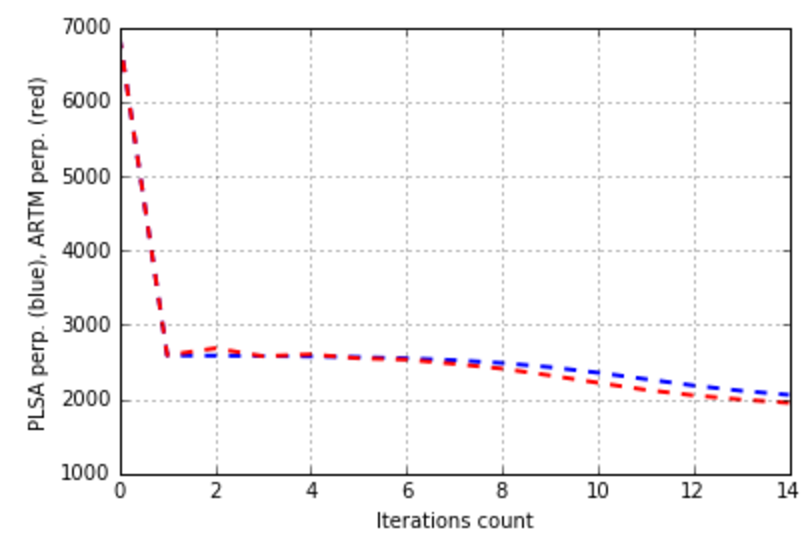
We can see, that we have an improvement of sparsities and kernel measures, and the downgrade of the perplexion isn’t big. Let’s try to increase the absolute values of regularization coefficients:
model_artm.regularizers['SparsePhi'].tau = -0.2
model_artm.regularizers['SparseTheta'].tau = -0.2
model_artm.regularizers['DecorrelatorPhi'].tau = 2.5e+5
Besides that let’s include into each model the artm.TopTokenScore measure, which allows to look at the most probable tokens in each topic:
model_plsa.scores.add(artm.TopTokensScore(name='TopTokensScore', num_tokens=6))
model_artm.scores.add(artm.TopTokensScore(name='TopTokensScore', num_tokens=6))
We’ll continue the learning process with 25 passes through the collection, and than will look at the values of the scores:
model_plsa.fit_offline(batch_vectorizer=batch_vectorizer, num_collection_passes=25)
model_artm.fit_offline(batch_vectorizer=batch_vectorizer, num_collection_passes=25)

print_measures(model_plsa, model_artm)
Sparsity Phi: 0.093 (PLSA) vs. 0.841 (ARTM)
Sparsity Theta: 0.000 (PLSA) vs. 0.023 (ARTM)
Kernel contrast: 0.640 (PLSA) vs. 0.740 (ARTM)
Kernel purity: 0.674 (PLSA) vs. 0.822 (ARTM)
Perplexity: 1619.031 (PLSA) vs. 1644.220 (ARTM)
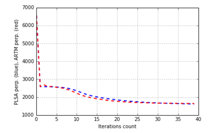
Becides let’s plot the changes of matrices sparsities by iterations:
plt.plot(xrange(model_plsa.num_phi_updates),
         model_plsa.score_tracker['SparsityPhiScore'].value, 'b--',
         xrange(model_artm.num_phi_updates),
         model_artm.score_tracker['SparsityPhiScore'].value, 'r--', linewidth=2)

plt.xlabel('Iterations count')
plt.ylabel('PLSA Phi sp. (blue), ARTM Phi sp. (red)')
plt.grid(True)
plt.show()

plt.plot(xrange(model_plsa.num_phi_updates),
         model_plsa.score_tracker['SparsityThetaScore'].value, 'b--',
         xrange(model_artm.num_phi_updates),
         model_artm.score_tracker['SparsityThetaScore'].value, 'r--', linewidth=2)

plt.xlabel('Iterations count')
plt.ylabel('PLSA Theta sp. (blue), ARTM Theta sp. (red)')
plt.grid(True)
plt.show()
The output:
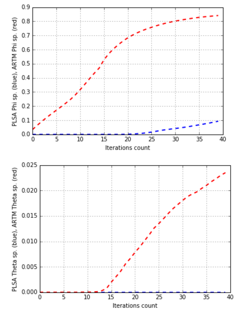
It seems that achieved result is enough. The regularization helped us to improve all scores with quite small perplexity downgrade. Let’s look at top-tokens:
for topic_name in model_plsa.topic_names:
    print topic_name + ': ',
    print model_plsa.score_tracker['TopTokensScore'].last_tokens[topic_name]
topic_0:  [u'year', u'tax', u'jobs', u'america', u'president', u'issues']
topic_1:  [u'people', u'war', u'service', u'military', u'rights', u'vietnam']
topic_2:  [u'november', u'electoral', u'account', u'polls', u'governor', u'contact']
topic_3:  [u'republican', u'gop', u'senate', u'senator', u'south', u'conservative']
topic_4:  [u'people', u'time', u'country', u'speech', u'talking', u'read']
topic_5:  [u'dean', u'democratic', u'edwards', u'primary', u'kerry', u'clark']
topic_6:  [u'state', u'party', u'race', u'candidates', u'candidate', u'elections']
topic_7:  [u'administration', u'president', u'years', u'bill', u'white', u'cheney']
topic_8:  [u'campaign', u'national', u'media', u'local', u'late', u'union']
topic_9:  [u'house', u'million', u'money', u'republican', u'committee', u'delay']
topic_10:  [u'republicans', u'vote', u'senate', u'election', u'democrats', u'house']
topic_11:  [u'iraq', u'war', u'american', u'iraqi', u'military', u'intelligence']
topic_12:  [u'kerry', u'poll', u'percent', u'voters', u'polls', u'numbers']
topic_13:  [u'news', u'time', u'asked', u'political', u'washington', u'long']
topic_14:  [u'bush', u'general', u'bushs', u'kerry', u'oct', u'states']
for topic_name in model_artm.topic_names:
    print topic_name + ': ',
    print model_artm.score_tracker['TopTokensScore'].last_tokens[topic_name]
topic_0:  [u'party', u'political', u'issue', u'tax', u'america', u'issues']
topic_1:  [u'people', u'military', u'official', u'officials', u'service', u'public']
topic_2:  [u'electoral', u'governor', u'account', u'contact', u'ticket', u'experience']
topic_3:  [u'gop', u'convention', u'senator', u'debate', u'south', u'sen']
topic_4:  [u'country', u'speech', u'bad', u'read', u'end', u'talking']
topic_5:  [u'democratic', u'dean', u'john', u'edwards', u'primary', u'clark']
topic_6:  [u'percent', u'race', u'candidates', u'candidate', u'win', u'nader']
topic_7:  [u'administration', u'years', u'white', u'year', u'bill', u'jobs']
topic_8:  [u'campaign', u'national', u'media', u'press', u'local', u'ads']
topic_9:  [u'house', u'republican', u'million', u'money', u'elections', u'district']
topic_10:  [u'november', u'poll', u'senate', u'republicans', u'vote', u'election']
topic_11:  [u'iraq', u'war', u'american', u'iraqi', u'security', u'united']
topic_12:  [u'bush', u'kerry', u'general', u'president', u'voters', u'bushs']
topic_13:  [u'time', u'news', u'long', u'asked', u'washington', u'political']
topic_14:  [u'state', u'states', u'people', u'oct', u'fact', u'ohio']
We can see, that topics are approximatelly equal in terms of interpretability, but they are more different in ARTM.
Let’s extract the matrix as pandas.DataFrame and print it (to do this operation with more options use ARTM.get_phi()):
print model_artm.phi_
                  topic_0   topic_1   topic_2   topic_3   topic_4   topic_5  \
parentheses       0.000000  0.000000  0.000000  0.000000  0.000000  0.000277
opinion           0.000000  0.000000  0.000000  0.000000  0.000000  0.000000
attitude          0.000000  0.000000  0.000000  0.000000  0.000000  0.000000
held              0.000000  0.000385  0.000000  0.000000  0.000000  0.000000
impeachment       0.000000  0.000115  0.000000  0.000000  0.000000  0.000000
...                    ...       ...       ...       ...       ...       ...
aft               0.000000  0.000000  0.000000  0.000000  0.000000  0.000419
spindizzy         0.000000  0.000000  0.000647  0.000000  0.000000  0.000000
barnes            0.000000  0.000000  0.000000  0.000792  0.000000  0.000000
barbour           0.000000  0.000000  0.000000  0.000000  0.000000  0.000000
kroll             0.000000  0.000317  0.000000  0.000000  0.000000  0.000000

                  topic_12      topic_13  topic_14
parentheses       0.000000  0.000000e+00  0.000000
opinion           0.002908  0.000000e+00  0.000346
attitude          0.000000  0.000000e+00  0.000000
held              0.000526  0.000000e+00  0.000000
impeachment       0.000000  0.000000e+00  0.000396
...                    ...           ...       ...
aft               0.000000  0.000000e+00  0.000000
spindizzy         0.000000  0.000000e+00  0.000000
barnes            0.000000  0.000000e+00  0.000000
barbour           0.000000  0.000000e+00  0.000451
kroll             0.000000  0.000000e+00  0.000000
You can additionally extract matrix and print it:
theta_matrix = model_artm.get_theta()
print theta_matrix
The model can be used to find  vectors for new documents via
 ARTM.transform() method:
test_batch_vectorizer = artm.BatchVectorizer(data_format='batches',
                                             data_path='kos_test',
                                             batches=['test_docs.batch'])
test_theta_matrix = model_artm.transform(batch_vectorizer=test_batch_vectorizer)
Topic modeling task has an infinite set of solutions. It gives us a freedom in our choice. Regularizers give an opportunity to get the result, that satisfacts several criteria (such as sparsity, interpretability) at the same time.
Showen example is a demonstrative one, one can choose more flexible strategies of regularization to get better result. The experiments with other, bigger collection can be proceeded in the same way as it was described above.
See Python Guide for further reading, as it was mentioned above.